PDE-Based Wave Simulation in Jetpack Compose: Canvas vs AGSL

  

In this article, I’ll build a 1D PDE wave simulation in Jetpack Compose, walk through performance tips and common pitfalls, and look at AGSL from a less obvious angle that is often missed at first glance.

Problem

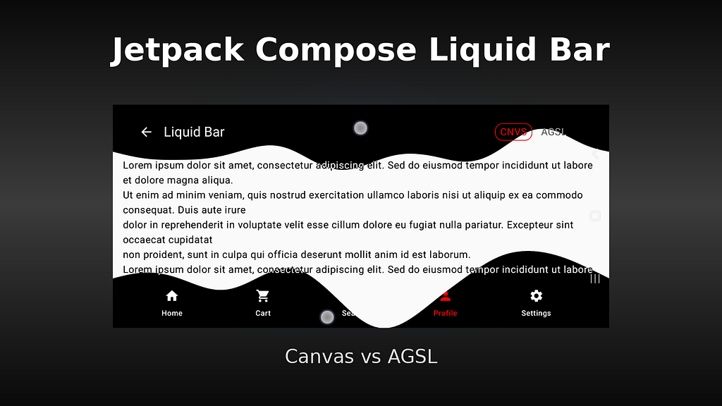
Let’s build an interactive liquid effect in Jetpack Compose: it reacts to touch, creates waves on the surface, slowly settles, and blends with real UI content like text and icons.
For blending, we want two behaviors: invert content colors in some areas or apply per-pixel alpha masking when content is partially covered by the wave.

The challenge is balancing visual quality and performance.
Effects like this can look great, but on Android they can also introduce jitter, delayed response, and extra redraw cost.

So the goal is practical: keep it responsive on real devices, reduce artifacts, and pick a rendering approach that stays stable under load.

The 1D Wave Model

For this effect, I use a 1D wave model based on the wave PDE (Partial Differential Equation). I won’t go into the full math derivation here and will focus on the implementation idea. In 1D, the wave is represented as a row of samples across the container width. Each sample stores vertical displacement (Y) at a specific horizontal position (X). At every frame, each point is updated from its two neighbors and its own value from the previous frame:

next[i] = (curr[i-1]+curr[i+1] — prev[i])*damping

Important detail: to compute the next state, we need both the current and previous states.
That is why the simulation keeps three buffers at the same time: prev, curr, and next (see Wave1D with three FloatArrays).
After each step, these buffers are rotated.

  internal class Wave1D(samples: Int) {
      ...
      private var curr = FloatArray(n)
      private var prev = FloatArray(n)
      private var next = FloatArray(n)
      ...
  }

Key wave parameters:
– samples — horizontal simulation resolution.
– damping — how quickly wave energy decays.
– yGain — visual wave amplification at render time.
– plotWidth — transition band width between the wave and non-wave space (hard vs soft edge).

Touches are handled as instant impulses. Each touch is clamped to valid X/Y bounds, converted to pulse strength, and distributed across nearby samples with touchPulseInfluence. We do not store touch paths; we only modify the current wave state at the moment of interaction, then continue with the same fixed-cost simulation step per frame. A key benefit of this approach is that even with many taps per second, the ongoing simulation complexity does not grow.

...
// Apply one touch impulse to the current wave state
fun inject(touchX: Float, touchYBottomUp: Float) {
      // 1) Normalize touch position and convert it to impulse strength
      val centerX = touchX.coerceIn(0.1f, 0.9f)
      val touchStrength = (1f - touchYBottomUp.coerceIn(0f, 1f)) * amp

      // 2) Spread that impulse across nearby wave samples
      // Iterate over all wave samples along X
      for (sampleIndex in 0 until n) {
          val sampleX = sampleIndex.toFloat() / (n - 1).toFloat()
          val influence = touchPulseInfluence(centerX, pulseWidthNorm, sampleX)
          if (influence != 0f) curr[sampleIndex] -= influence * touchStrength
      }
  }
...

where toushPulseInflience() computes how much each sample is affected by the touch, based on distance from the touch center: maximum influence near the center, smoothly fading to zero within pulseWidthNorm

Main touch-tuning parameters:
– amp — impulse strength injected by touch.
– pulseWidthNorm — horizontal width of the touch influence zone.
– dragThrottleMs — injection rate limit during drag (lower value = more frequent injections).

At each frame tick, we run Wave1D.step().
Inside this function, we update every sample point using its neighbors and compute the next wave state.
After that, we swap buffer roles: the current state becomes previous, and the newly computed state becomes current.

fun step() {
      for (i in 1 until n - 1) {
          next[i] = (curr[i - 1] + curr[i + 1] - prev[i]) * damping
      }

      // Swap roles: prev <- curr, curr <- next
      val oldPrev = prev
      prev = curr
      curr = next
      next = oldPrev
  }

This way, the next frame always starts with fresh wave data instead of rebuilding arrays from scratch.

Common Runtime Model

So the Update-Render Loop is:

• Frame tick
• Wave1D.step() updates wave swap buffers
• draw wave (Canvas or AGSL)
• Frame tick (repeat)

Each LiquidBox (top and button bar) is intentionally taller than the visible bar area: the top container is about twice the top bar height, and the bottom container is about about twice the bottom bar height. Both containers overlap the scrolling content. This extra height gives the wave enough vertical space to breathe and animate naturally, while only the bar zone remains interactive.

Well, during development AGSL RenderEffect Approach was my favorite approach, so I was focusing on it . At the same time, I also optimized the Canvas approach, even though I was not very motivated, mainly to make sure this option was covered but the final results turned out to be different from my initial
expectations.

Common Optimization Pitfalls and Performance Tips

State Handling (Mutable Buffers Over Immutable State):
In typical Android/Kotlin UI, immutable state and data-class copies are often preferred. For high-frequency simulation, that approach is too expensive. Creating new objects every frame adds avoidable allocation and GC pressure, so this solver keeps mutable numeric buffers and updates them in place. That keeps per-frame work significantly cheaper.

In typical Android/Kotlin UI, immutable state and data-class copies are often preferred. For high-frequency simulation, that approach is too expensive. Creating new objects every frame adds avoidable allocation and GC pressure, so this solver keeps mutable numeric buffers and updates them in place. That keeps per-frame work significantly cheaper.

Reduce simulation samples count:
The wave solver keeps three buffers (prev, curr, next), each with length = samples. For example, with a 1024px container, you can reduce samples from 1024 to 126 to lower simulation cost.

So sample count should directly affect step() performance, because step() iterates over wave samples every frame.
That is exactly what the experiment showed:

At samples = 126, step() took about 31–43 µs (~0.03–0.04 ms).
At samples = 2024, it increased to about 500–1050 µs (~0.5–1.05 ms) — roughly 15–25x slower, with near-linear scaling.

So yes, higher sample count clearly increases simulation cost. But even in the high-sample case, step() stayed up to ~1 ms, which is still a relatively small part of a 16.6 ms frame budget.

Interpolation:
Because the wave is sampled, a low sample count can make the shape look stair-stepped, like a bar chart. To avoid this, interpolation should be applied during rendering.

• 2-tap linear interpolation: low cost and usually good visual quality.
• 3-tap smoothing filter: smoother than linear, with a small extra cost.
• 4-tap cubic interpolation: smoother curves, but more expensive and harder to tune.

Use drawWithCache over remember(…):
For both Canvas and AGSL-Canvas paths, drawWithCache is usually a better fit for render resources.
It keeps objects at draw-node level, such as Paint, shader instances (RuntimeShader, BitmapShader), and helper path data. When a draw modifier depends on frame-driven state (for example, frameTick), using remember(…) can recreate the draw node on every tick, which adds modifier-chain churn instead of only triggering redraw. drawWithCache keeps the draw node stable and re-runs only the draw callback, so each tick triggers redraw rather than draw-node recreation.

Reduce Per-Frame Updates (Not Recommended):
In theory, updating simulation and rendering less often should reduce frame cost. In practice (my case), it did not improve the expensive frames and introduced visible stutter. This approach creates perceived FPS drops and hurts visual quality, so it should be avoided.

Avoid Too Many Heavy Animated Containers on One Screen:
When several containers run heavy per-tick work on the same screen, frame-time spikes become much more likely. If multiple animated zones are required, try to share rendering passes or reduce overlapping expensive effects. Even when simulations remain separate, reducing pipeline overhead (extra layers/compositing) can still improve stability.

Stop the Simulation When the Wave Has Settled:
When the wave is no longer moving, there is no reason to keep ticking and redrawing the same state. You can also increase damping so the wave settles faster and the animation runs for less time.

In this project, each step() evaluates the current “energy value” (maxAbsNext) and its frame-to-frame change (maxDelta). When both stay below the rest threshold for several consecutive frames, the simulation stops running.

Prefer built-in optimized rendering primitives over custom loops :
Whenever possible, use standard GPU-optimized APIs (drawPath, shader interpolation via mix/smoothstep, and drawWithCache) instead of manual per-pixel/per-column drawing logic.

AGSL RenderEffect

Uses RuntimeShader through RenderEffect as a post-processing pass on the LiquidBox layer. The shader itself is straightforward: it samples a 1D wave profile, builds a per-pixel wave mask, and composites liquid
color with source content.

Main uniforms passed to AGSL:

• container size (uContainerWidthPx, uContainerHeightPx)
• profile width (uProfileWidthPx)
• band/thickness (uBandPx)
• orientation (uIsTop)
• liquid color (uWaveColor)
• profile texture (waveProfile)

Because we cannot run persistent PDE simulation state directly inside this shader (no shared mutable simulation buffer/output feedback loop), wave state is computed on CPU and uploaded each frame. AGSL does not
accept raw arrays directly, so the wave samples are packed into a 1 x N bitmap (N = sample count)

Encoding note:

• 8-bit in one channel is possible for coarse values.
• For precise per-pixel height, two channels are used (RG = 16-bit packed value), which is enough precision for screen-space wave height mapping.

In this project, each wave sample height is converted to a 16-bit value before being sent to AGSL. This is handled by rememberWaveProfileArgb16(): the normalized height is quantized to 0..65535, then packed into two bitmap channels (Red = high byte, Green = low byte).
So the profile texture is 1 x N, and each texel stores one sample with 16-bit precision using two channels, not one.

If needed, this can be reduced to a single channel, but the gain is usually small because the bitmap dimensions stay the same.

The bigger win comes from moving interpolation to AGSL: instead of expanding data to full container width on CPU, we upload only N simulation samples. Otherwise, we would have to prepare and upload a profile with width equal to container pixels (often around 1060 in portrait on many phones).
Among the available AGSL interpolation options, 2-tap linear interpolation (mix) was used. This option is cheap and gives good visual quality.
smoothstep shaping was not used, because UI element boundaries are intentionally sharp, and a soft transition would look inconsistent with standard Android UI elements such as the top app bar and bottom app bar.

Because RuntimeShader via RenderEffect works as a post-processing pass, it allows cheap per-pixel checks during shader evaluation. Each pixel can be tested against the wave level, and top/bottom app bar UI pixels (tabs, text, buttons, icons) above the wave can be filtered out by reducing alpha (pixel-level alpha filter). This per-pixel filtering over the layer content is a key feature of the RenderEffect approach:

In theory, RuntimeShader supports dynamic uniform updates via setFloatUniform. However, when it is used through RenderEffect in a Compose graphicsLayer, uniform updates alone often do not trigger redraw. As a result, RenderEffect is frequently recreated to force layer refresh, which introduces extra allocations during frame updates.

AGSL via Canvas (RuntimeShader + Paint)

AGSL-in-Canvas was used as a hybrid renderer: Wave1D stays on CPU, while AGSL handles final pixel shaping on GPU via Canvas shader drawing. In this setup, it reduced some RenderEffect overhead and kept frame updates more predictable, while preserving visual quality through shader-side interpolation.

The key difference from Runtime RenderEffect is that this shader is rendered as an explicit overlay layer, rather than applied as a post-processing effect.

Compared to the Runtime RenderEffect path, this AGSL-in-Canvas variant does not require recreating the shader object each frame, which keeps update flow simpler.

However, wave-boundary pixel filtering of underlying UI elements (like in the Runtime post-processing approach) is harder to implement here, because it requires additional layer/blend orchestration. This is not
implemented in this project.

This approach also relies on AGSL’s built-in GPU pipeline, so it remains highly optimized and is typically on par with Runtime RenderEffect. In some cases, it can even be faster.

Classic Canvas Renderer

In a pure Canvas renderer, the wave can be drawn as vertical drawRect columns, but this is heavier and often looks stepped. To smooth it out, you would need to increase fragment count and interpolate closer to
screen-pixel width, which quickly raises per-frame draw cost…

But there is a more powerful option: Path API. No extra fragment upscaling or manual interpolation is needed here. Path APIs already include built-in curve primitives (quadraticBezierTo / cubicTo), so one smooth wave path can be built and rendered in a single pass, with good visual quality and solid performance.

Another nice thing about Path API is that clipping by path is straightforward: clipPath(…) { drawContent() }. It helps solve content overlap when UI elements cross the wave boundary. In the Runtime RenderEffect approach, this was handled with per-pixel alpha filtering instead.

Results and Comparison (HWUI Profiling)

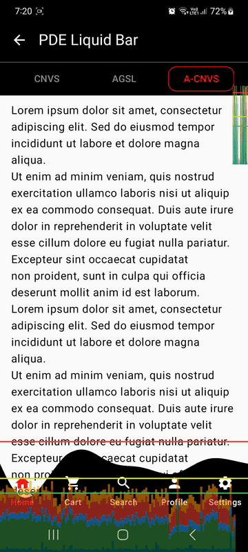
In my measurements, all variants stayed below the red line, but AGSL Runtime RenderEffect was the slowest.
The Canvas renderer performed best and stayed closer to the green line, (even with additional costs enabled (either clipPath or full-screen Difference blend via offscreen graphicsLayer for UI color inversion).

In AGSL Runtime RenderEffect mode, the blue Draw segment is mostly gone, while the orange Swap segment becomes larger. This indicates that frame cost shifts from CPU draw work to GPU present/synchronization, so
more time is spent waiting at eglSwapBuffers before the frame is shown.

A control test with an almost empty screen and a trivial per-frame AGSL shader (solid color only) showed similar HWUI bar heights. This suggests the main cost comes from the RuntimeShader/RenderEffect pipeline
itself, so extra micro-optimizations in this AGSL Runtime path are unlikely to matter much.

Why did Canvas win here?
In this case, Compose only issues draw commands, while Path building/rasterization runs in the native graphics stack (Skia/C++).
A Path-based wave is then rendered as geometry, mostly over the shape area. By contrast, the AGSL Runtime RenderEffect path applies shader
work over the whole target layer (effectively a per-pixel pass), which increases GPU present/sync cost.
So for this effect, drawPath turned out faster and more stable than full-layer AGSL post-processing.

Final Takeaways

• For frame-ticked, physics-heavy one-dimensional simulations without advanced pixel effects, sampling with classic Canvas Path rendering is usually the best practical choice. In this case, per-pixel AGSL
  Runtime RenderEffect did not provide a performance win in this case.
• AGSL Runtime RenderEffect can produce very powerful per-pixel visuals, and it shines when complex texturing or shader-only effects are needed. The downside is data flow: complex effects usually require complex state models, and updating/managing that state every frame can become a bottleneck. In AGSL, dynamic data is often packed into bitmaps (up to 4 channels × 8 bits per pixel) and uploaded per frame, which adds CPU/GPU transfer cost. Unlike OpenGL/Vulkan GLSL pipelines (with persistent GPU buffers and ping-pong resources), AGSL RuntimeShader does not expose writable/shared GPU buffers for simulation state. Because of that, heavy state updates stay CPU-driven and can hurt frame time.
  A buffered-state API in AGSL would significantly improve this kind of workload.

Source code: GitHub link to the current project.

Thanks:)

---

PDE-Based Wave Simulation in Jetpack Compose: Canvas vs AGSL was originally published in ProAndroidDev on Medium, where people are continuing the conversation by highlighting and responding to this story.